Documentation
Getting Started
Installation and start-up
- If not already installed, download and install Chimera. Sophia has been tested with Chimera v1.8 and higher. ChimeraX, the next generation of Chimera, is not currently supported.
- Go to the Sophia home page. Click download button.
- Unzip Sophia.
- Launch Chimera
-
Click
Fileand thenOpen…. -
Navigate to the Sophia directory and select
launch_sophia.py. - Click the Sophia icon. It should appear in the toolbar on the left side of the main Chimera window. (Note: in the screenshot below, we’ve already loaded a system of argon atoms; your window will be empty initially).
Visualization Presets
Sophia comes with several visual style presets, but in order to use them, you must first tell Chimera where to find them:
-
In Chimera, click
Presetsand thenAdd Custom Presets…. - In the Preferences window that appears, click the “Add…” button.
-
Navigate to the Sophia directory and select the
CustomPresetssubdirectory. - In the Prefences window, click the “Save” button and then the “Close” button.
-
Now, if you click
Presetsin Chimera, there should be several new entries to choose from:Custom 1 (SophiaLicorice)andCustom 2 (SophiaVDW).
Basic Concepts
Simulation
In Sophia, a Simulation is made up of three things:
- Universe (what to simulate)
- Recipe (how to simulate it)
- Trajectory (the result of carrying out the Recipe)
Universe
The Universe is the physical system being simulated. It includes the atoms and molecules in the system, as well as the force field (energy function) that describes their interactions.
Recipe
The Recipe is the set of instructions for carrying out the simulation. We refer to each step of the Recipe as an Ingredient. Here's what a sample Recipe might look like:
- Run Molecular Dynamics for 10000 steps, heating from T=1K to T=100K.
- Run Molecular Dynamics for 10000 steps, hold T at 100K.
- Minimize using Steepest Descent for 1000 steps.
(But, actual recipes are not this verbose. They are represented in JSON format, instead of plain English.)
Trajectories and epochs
The Trajectory is the output obtained by carrying out the Recipe on the Universe. We refer to each segment of the trajectory as an Epoch. Each Epoch corresponds to an Ingredient in the Recipe.

User Interface
Main Window
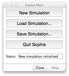
The Main Window allows you to start new simulations, as well as load and save them. This window also reports the status of Sophia.
- New Simulation: Clears any existing data and initializes Sophia.
-
Load Simulation: Load a previously saved simulation. You must select the
.sophiafile that was created when you saved. -
Save Simulation: Save the current simulation. When prompted, navigate to the directory where you would like to save your simulation. Enter a name for the simulation. Sophia saves several files together, but each one will contain the name you specify as a prefix. To load later, you will need to select the
your_prefix.sophiafile. - Quit Sophia: Clear existing data and close all Sophia windows, returning the user to Chimera.
Universe Window
The Universe Window is used when creating a new simulation. The input fields are:
- PDB File: click the button and then select a PDB file.
- Force Field: choose from LennardJones, Amber94, Amber99, or GAFF (Generalized Amber Force Field). LennardJones is mainly used for simple atomic simulations, like a box of argon atoms. Amber94 and Amber99 are used for peptides, proteins, and nucleic acids. GAFF is used for small molecule simulations, such as ethane or butane.
-
FF Mod File: the FF Mod File will modify the default force field parameters. It is optional. Click the button and then select a .frcmod file (for Amber or GAFF simulations) or a .mod file (for LennardJones simulations).
Format of .mod files
--------------------
Ar, 4.8, 0.3
(atom name), (well depth (kJ/mol)), (R_min (nanometers))

Format of .frcmod files
-----------------------
bond modification format:
(atom names) (force constant) (equilibrium bond length (angstroms))
example: c3-c3  635.8    1.5400

dihedral modification format:
(atom names) (divide barrier by this quantity) (0.5 * energy barrier (kcal/mol)) (phase shift angle (degrees)) (periodicity)
example: hc-c3-c3-hc   1    0.00          0.0             3.

van der Waals modification format:
(atom name) (vdw radius (angstroms)) (well depth (kcal/mol))
example:  c3          1.3000  0.1000
The .frcmod format is described in more detail in the Amber documentation. - Box Length: the length of the periodic bounding box. Atoms that pass through the edge will reappear on the other side of the box. Setting this value to zero or negative values will instead create a Universe with no bounding box, i.e. atoms can drift away to infinite separation. Currently, the only available options are: periodic boundary or no boundary.
- Non-bond Cutoff: non-bonded interactions (electrostatic and van der Waals) will not be computed for pairs of atoms separated by greater than this distance.
- Load Universe: after configuring the fields above, click this button to load the Universe.
- Reset Universe: refresh Universe to original state. Any changes since loading the Universe will be wiped out, including any recipe or trajectory data (so use with caution!).
Recipe Window
The Recipe Window has two panels:
-
Recipe Panel
- This panel lists the Ingredients of the simulation.
- You can save/load recipes using the buttons at the top of the panel.
-
The buttons at the bottom of the panel allow you to:
- Move an existing ingredient up or down in the recipe.
- Initialize a new ingredient.
- Clone an existing ingredient.
- Delete an existing ingredient.
-
When running a simulation, the status of each Ingredient will change from
InitializedtoRunningand then finally toDone. When an Ingredient isDone, it can no longer be deleted. It becomes a permanent part of the history of the simulation.
-
Ingredients Panel
-
When you select an Ingredient in the
Recipe Panel, the parameters that correspond to that ingredient will appear in theIngredients Panel. -
Use the
Ingredients Panelto change the parameter values of the currently select Ingredient. - To change the algorithm of an Ingredient, click on the desired tab (MD for Molecular Dynamics or EM for Energy Minimization).
-
When you select an Ingredient in the
The Ingredients Panel has four tabs:
-
MD (Molecular Dynamics)
- Num Steps: the number of MD steps to run
-
Output Interval: record energy and coordinates after every
Output Intervalnumber of steps - Time Step: number of femtoseconds per step
- Initialize Velocities: assign random initial velocities in the x, xy, or xyz dimensions
- Thermostat: adjust temperature by rescaling velocities or adding a Nose thermostat; must use rescaling to raise or lower temperature – use Nose to maintain constant T
- Initial Temperature: starting temperature in Kelvins
-
Final Temperature: ending temperature in Kelvins; velocities will be linearly rescaled over the course of
Num StepsfromInitial TemperaturetoFinal Temperature(but only ifThermostatis set toRescale) -
Rescale Interval: rescale velocities after every
Rescale Intervalnumber of steps (but only ifThermostatis set toRescale) -
Nose Thermostat Relaxation Time: the relaxation time of the thermostat coordinate (only used if
Thermostatis set toNose) -
Barostat: used to enable Andersen barostat to regulate pressure in NPT simulations (requires
Box Length > 0) -
Pressure: pressure of the simulation, enforced by Andersen barostat if
Barostatis set toAndersen -
Andersen Barostat Relaxation Time: the relaxation time of the barostat coordinate (only use if
Barostatis set toAndersen) -
Remove Translation Interval: subtract the total velocity of the system from each atomic velocity after every
Remove Translation Intervalnumber of steps -
Remove Rotation Interval: adjusts the atomic velocities such that the total angular momentum is zero after every
Remove Translation Intervalnumber of steps
-
EM (Energy Minimization)
- Algorithm: SD (Steepest Descent) or CG (Conjugate Gradient)
- Num Steps: the number of EM steps to run; might stop terminate early if convergence criterion is satisfied
-
Output Interval: record energy and coordinates after every
Output Intervalnumber of steps - Initial Step Size: length scale of first trial move; the step size will be dynamically adjusted as the minimization continues
-
Convergence: halt minimization before
Num Stepsare complete if successive steps change the gradient by less than this amount (the field is asking for the exponent)
-
MC (Monte Carlo)
- Num Steps: the number of MC steps to run
-
Output Interval: record energy and coordinates after every
Output Intervalnumber of steps - Initial Step Size: length scale of first trial move; the step size will be dynamically adjusted as the minimization continues
- Initial Temperature: starting temperature in Kelvins
-
Final Temperature: ending temperature in Kelvins; velocities will be linearly rescaled over the course of
Num StepsfromInitial TemperaturetoFinal Temperature
-
LD (Langevin Dynamics)
- Num Steps: the number of MD steps to run
-
Output Interval: record energy and coordinates after every
Output Intervalnumber of steps - Time Step: number of femtoseconds per step
- Initialize Velocities: assign random initial velocities in the x, xy, or xyz dimensions
- Friction: when this parameter is 0, the simulation will behave like molecular dynamics; when this parameter is large, the simulation will behave like brownian dynamics
- Thermostat: adjust temperature by rescaling velocities or adding a Nose thermostat; must use rescaling to raise or lower temperature – use Nose to maintain constant T
- Initial Temperature: starting temperature in Kelvins
-
Final Temperature: ending temperature in Kelvins; velocities will be linearly rescaled over the course of
Num StepsfromInitial TemperaturetoFinal Temperature(but only ifThermostatis set toRescale) -
Rescale Interval: rescale velocities after every
Rescale Intervalnumber of steps (but only ifThermostatis set toRescale) -
Nose Thermostat Relaxation Time: the relaxation time of the thermostat coordinate (only used if
Thermostatis set toNose) -
Barostat: used to enable Andersen barostat to regulate pressure in NPT simulations (requires
Box Length > 0) -
Pressure: pressure of the simulation, enforced by Andersen barostat if
Barostatis set toAndersen -
Andersen Barostat Relaxation Time: the relaxation time of the barostat coordinate (only use if
Barostatis set toAndersen) -
Remove Translation Interval: subtract the total velocity of the system from each atomic velocity after every
Remove Translation Intervalnumber of steps -
Remove Rotation Interval: adjusts the atomic velocities such that the total angular momentum is zero after every
Remove Translation Intervalnumber of steps
Trajectory Window
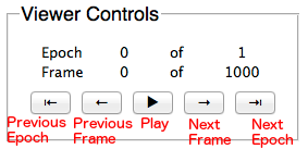
Use the Trajectory Window to navigate between the frames and epochs of a simulation. Note: the frames and epochs are 0-indexed, so “0 of 1” means there are two epochs: epoch 0 and epoch 1.
Energy Plot Window
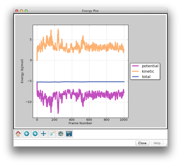
The Energy Plot Window shows the potential, kinetic, and total (potential + kinetic) energies from the currently loaded simulation. The dark vertical line marks the frame that you are currently viewing. The light gray vertical lines mark epoch boundaries. Clicking on the Previous Epoch and Next Epoch buttons in the Trajectory Window will jump to the nearest epoch boundary in the reverse or forward direction, respectively. The icons along the bottom row of the plot allow you to zoom in/out and save the plot to a png file. From left to right, the icons are:
- Home icon: jump to original view
- Back icon: jump to previous view
- Forward icon: jump to next view
- Arrows icon: translate point of view
- Magnifying glass icon: highlight a region and zoom in
- Square with green arrows icon: adjust aspect ratio of plot
- Disk icon: save plot to .png
Note: when playing a trajectory, plot animations will only function properly in the original view. If you zoom in, the animations will not render correctly. You can always return to the original view by clicking the Home icon.
Structural Measurements
After running a simulation, click on the “Structure Measurements…” button in the Trajectory Viewer window. That pulls up a Chimera dialog that lets you define distances and angles that you want to measure. Control-shift click on each atom of interest and then click “Create” in the Chimera dialog to define a distance or an angle.
After you’ve defined your selections, click the check boxes in Sophia’s Trajectory Viewer window to plot your selected (pseudo)bonds or angles/torsions. When you save a simulation, any distances or angles that have been defined will automatically be saved to file (epoch00_bonds.csv, epoch01_bonds.csv, etc.)
Examples
Running an argon simulation
-
With Chimera open and Sophia loaded, click
New Simulationin theMain Window. TheUniverse Windowwill appear. -
Click
Load PDB File. Navigate to the Sophia directory and then to thePDBsubdirectory. Select eitherargon.pdborargon2.pdb. -
Set
Force FieldtoLennard Jones, and then clickLoad Universe. -
If you’ve loaded Sophia’s visual presets, you can click
Presetsand select theSophiaVDWpreset for a useful van der Waals representation of the argon atoms. -
In the
Recipe Window, clickNewto create a new Ingredient. When you clickNew, the algorithm of the new ingredient will match the tab that is currently selected in theIngredients Panel. -
To modify the parameters of the new ingredient, first select the ingredient by clicking on it in the
Recipe Panel. Then, use theIngredients Panelto change the parameters. Click on a different tab in theIngredients Panelwill change the algorithm of the selected ingredient. -
An alternative to the previous two steps would be to load a saved recipe, rather than creating a new one. To do so, you would click
Load Recipeand select a recipe from theRecipesdirectory, included with Sophia. -
You can duplicate existing ingredients by selecting them in the
Recipe Paneland clicking theClonebutton. Likewise, theDeletebutton will remove the selected ingredient. -
When you’ve finished building/loading the simulation recipe, click
Run All Ingredients. Alternatively, you can click theRun Next Ingredientbutton, and the simulation will stop and wait for your input after one ingredient has been completed. -
When the simulation is complete, the trajectory will be loaded for viewing. Use the
Trajectory Viewerwindow to play the movie or advance by frame or by epoch. -
To save the simulation, click
Save Simulation…in theMain Window. Navigate to the directory where you would like to save your simulation. Enter a name for the simulation. Sophia saves several files together, but each one will contain the name you specify as a prefix. -
You may return to Chimera by clicking
Quit Sophia. -
It's also possible to add more ingredients and click
Run All Ingredientsagain to add more epochs to the trajectory. Note: clicking Run won’t redo the ingredients you’ve already completed; it will only run ingredients that are not yet done.
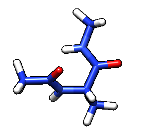
Running an alanine simulation
Follow the argon procedure except for two changes:
-
In step 2, load
bALA1.pdb. -
In step 3, select
Amber94orAmber99as the force field. -
For better viewing, click
Presetsin the Chimera window and selectSophiaLicorice. You should see a representation similar to this: