Tutorial 6 Ten Atoms of Lennard-Jonesium: Energy Minimization
6.1 Introduction
“Energy minimization” refers to molecular mechanics algorithms aimed at reducing the potential energy of a collection of atoms. In this tutorial, you will examine two common minimization algorithms, steepest descent and conjugate gradient.
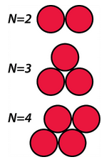
You will carry out a series of minimizations on different configurations of ten atoms of Lennard-Jonesium in two dimensions. The tutorial is limited to two dimensions, because this makes it very easy to examine the structures. (In two dimensions, the spherical atoms look and behave like disks.) We use Lennard-Jonesium, because the minimum energy structure is the configuration that maximizes the number of interatomic contacts. In the optimum configuration in two dimensions, two LJ atoms have one contact, three atoms have three contacts, and four atoms have five contacts (see figure).
6.2 Prediction
What is the minimum energy configuration of ten LJ atoms in two dimensions? From the discussion in the previous paragraph and the figure, you can see that you can tackle this problem by using ten coins on a table. Explore this conformational space and see if you can figure out what the optimum configuration of ten LJ atoms is. Draw a sketch of what you believe to be the optimum structure.
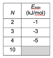
Count the contacts. In this tutorial, you will use an energy function that gives E = -1 kJ/mol for each ideal contact. The energy of a configuration with c contacts is thus predicted to be -c (kJ/mol). The predicted energies of the ideal conformations for the cases shown in the figure above are given in the table below. (N is the number of atoms.) There is also a space for you to enter your prediction for the energy of the optimum conformation of ten atoms of Lennard-Jonesium.
6.3 Setup and run first simulation
Create a new folder for your work on this tutorial.
Open Chimera, Launch Sophia, and initiate a new simulation with:
- PDB File: LJ10-2.pdb
- Force Field: Lennard-Jones
- FF Mod File: LJ_E0_1.0.frcmod
- Box length: 2 nm
- Non-bond cutoff: 1 nm
Click on “Load Universe”
In the Sophia Recipe Window:
- Recipe…: SD_1000x1_conv_E-6.json
To run the simulation, highlight the first ingredient in the Sophia Recipe Window – it will turn blue – and click “Run Next Ingredient”.
The recipe specifies steepest descent minimization, with the trajectory terminating after 1000 steps or upon satisfaction of the convergence criterion, whichever comes first. “conv_E-6” in the name of the recipe means that convergence is reached when a step produces a fractional change in energy less than one part in 1,000,000.
6.4 Analysis of first simulation
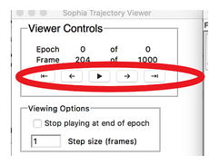
Adjust the display so the Chimera window, the Trajectory Viewer and the Energy Plot are all visible. The controls in the Trajectory Viewer allow you to move forward and backward in the simulation.
Play the trajectory and watch both the changes in energy and the changes in atomic positions. Answer the questions below:
Count the number of inter-atomic contacts in the final structure. Does it match your prediction? If so, does the final energy match your prediction?
Does the final structure correspond to the global minimum? If not, is the structure at a local minimum?
Did the minimization satisfy the numerical convergence criterion?
Based on your answers to the previous three questions, carefully explain in what sense the simulation has converged, and in what sense it has not converged.
6.5 Other simulations
Quit Sophia. Then re-launch it and repeat the previous exercise, using the structure in LJ10-3.pdb.
Comment on the ways this simulation does or does not converge.
LJ10-3.pdb differs from LJ10-2.pdb by only a small difference in the position of atom 6. Why does the final structure differ so much from that of the previous simulation?
Once again, this tutorial demonstrates how a relatively small difference in two structures can produce quite large differences in the results of a simulation.