Tutorial 5 Ten Atoms of Lennard-Jonesium: MD Simulation
5.1 Introduction
The purpose of this tutorial is to introduce you to MD simulations on systems containing more than two atoms. To make it easy to visualize the trajectory and to interpret the system’s behavior, we use a two-dimensional system with only ten atoms of Lennard-Jonesium.
You will run a free molecular dynamics simulation. By “free”, we mean that the atoms are all initially at rest, that they begin to move as a consequence of the forces between them, and that the system’s trajectory is entirely a consequence of its initial configuration, the inter-atomic forces, and the effects of inertia.
You will also be asked to predict how the system will behave. The initial configuration looks like a snapshot of a gas – the atoms are not clustered as they would be in a liquid or a solid. But the initial velocities of the atoms are all zero, and they are attracted to one another by the van der Waals forces. Will the system remain a gas, or will it condense into a liquid-like or solid phase?
5.2 Getting Ready
Create a new folder for your work on this tutorial. You’ll need the following files:
- PDB Files: LJ10-0.pdb and LJ10-1.pdb
- FF Mod Files: LJ_E0_0.1.frcmod
- Recipe: LJ10_MD.json
Before you load these into Sophia, double-click on LJ10.pdb. This should cause Chimera to open and display the initial configuration. (If it doesn’t, open Chimera and load LJ10.pdb.) Change the atomic representation to Spheres to see the initial configuration.
Throughout this tutorial, do NOT rotate the structure in the Chimera window. This is a two-dimensional system, and \(z = 0\) for all atoms throughout the trajectory. If you rotate the structure, you may create the impression that some pairs of atoms are overlapping, when they are not actually doing so. You can reset the view by clicking the Reset View button next to the Sophia logo on the toolbar.
5.3 Prediction
At the start of the simulation (\(t = 0\)), all the atoms are at rest. You are to guess what will happen as time passes.
As before, it doesn’t matter whether your guess is right or not – what’s important is for you to think about the likely behavior of the system. This will help you understand the results of the simulation once it’s been run.
There is no way to predict the trajectory (the atomic positions) of the entire system, because there are so many degrees of freedom. Nor can we predict the trajectory of a single atom, because that depends on the positions and motions of the other nine atoms.
However, there is one thing that you can predict, at least for the case where all the initial velocities are zero: how the potential, kinetic and total energies will evolve with time. No one can predict the exact behavior of these three inter-related quantities over a long time. But you should be able to make a qualitative prediction about their behavior at the very beginning of the simulation: will each of these increase, decrease, or remain constant? And you should be able to make a qualitative prediction about how they will behave after the system has come to equilibrium, which occurs within about 100-200 steps (10-20 ps).
To make your prediction more specific:
Draw a sketch showing your expectations for \(E_p(t)\), \(E_k(t)\) and \(E_{tot}(t)\). You can make a single sketch that describes both their initial evolution and their behavior after equilibrium is reached, or you can make two separate sketches. Remember that you are describing the case where all the initial atomic velocities are zero.
Write brief statements explaining the reasons for your predictions.
Now, before opening Sophia, quit Chimera, to clear all its settings.
5.4 Setup the first simulation and run it
Open Chimera, launch Sophia, and initiate a new simulation.
In the Sophia Universe window:
- PDB file: LJ10-0.pdb
- Force field: Lennard-Jones
- FF Mod file: LJ_E0_0.1.frcmod
- Box length: 10 nm
- Non-bond cutoff: 2 nm
- Click on “Load Universe”
Chimera: Actions / Atoms/Bonds / sphere
Sophia Recipe window:
- Load recipe: LJ10_recipe.json
- Highlight the recipe and run it.
This should generate a trajectory covering 100 ps, with output interval = 0.1 ps (1000 frames).
5.5 Analysis
Set up your screen so you can see the Chimera window, the Sophia Energy Plot window, and the Sophia Trajectory Viewer window simultaneously.
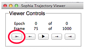
Using the Viewer Controls in the Sophia Trajectory Viewer window, watch the first ~50-100 frames of the trajectory. Pay attention to the atomic motions in the Chimera window, and to the plots of \(E_p\), \(E_k\) and \(E_{tot}\). You can play this part of the trajectory several times by using the reset button in the Sophia Trajectory window, shown below. (You can hit the reset button at any time; you don’t have to wait for the trajectory to finish.)
Describe the atomic motions and the changes in \(E_p\), \(E_k\) and \(E_{tot}\) in the first ~50-100 frames of the trajectory.
If there are any differences between your predictions and the observed behavior, explain why the system behaves differently from your predictions. (Write down your explanation.)
Describe the atomic motions and the changes in \(E_p\), \(E_k\) and \(E_{tot}\) during the part of the trajectory after the system has reached equilibrium.
If there are any differences between your predictions and the observed behavior, explain why the system behaves differently from your predictions. (Write down your explanation.)
Generate a plot showing how the temperature changes with time. You can do this by clicking on “Temperature” in the Plotting Options panel in the Sophia Trajectory Viewer window.
Describe how the temperature behaves in the first ~50-100 frames and write an explanation of this behavior.
Why does the temperature fluctuate after the system reaches equlibrium, instead of remaining constant?
Save the simulation. (Click on “Save Simulation” in the Sophia Main window; then go to the folder you created for this tutorial.)
Take snapshots of the energy plot, and of the structure at the final frame of the simulation (instructions here). You will need these in order to answer the questions below.
5.6 Repeat the simulation
Reset the system by clicking “Reset Universe” in the Sophia Universe window.
Using exactly the same parameters as before, reload the files, and rerun the simulation.
Do you get the same results, or different results? Explain.
5.7 Repeat the simulation with a slightly different starting conformation
Reset the system by clicking “Reset Universe” in the Sophia Universe window.
Run a new simulation, identical to the previous one, except using LJ10-1.pdb for the starting conformation.
How does the trajectory with this conformation differ from the trajectory with LJ10-0?
Take snapshots of the energy plot, and of the structure at the final frame of the simulation (\(t = 100\) ps) for the LJ10-1 simulation.
To explain how the two simulations differ, you will want to refer to the snapshots from each simulation, and you will need to open the two PDB files in a text editor.
Answer the following questions:
- What is the difference in the structures of the two conformations?
- What is the difference in the energies of these two conformations?
- Why do the two conformations produce such different MD trajectories?
A relatively small change in the initial structure can produce quite large differences in the final structure.