Tutorial 2 Analyzing the Accuracy of the Harmonic Oscillator MD Simulation
2.1 Introduction
In this tutorial, you will analyze the trajectory of the MD simulation carried out in Tutorial 1. The harmonic oscillator in that simulation consists of a mass m connected to a fixed point by an ideal Hookean spring with force constant \(k\) and ideal length \(x^*\). Its potential energy is
\[\begin{equation} E_p(x) = \frac{1}{2}k(x - x^*)^2 \tag{2.1} \end{equation}\]
and the period of its motion is
\[\begin{equation} T = 2 \pi \sqrt{m/k} \tag{2.2} \end{equation}\]
2.2 Preparation
- Calculate the period of the harmonic oscillator using Equation (2.2). The system in Tutorial 1 had an atomic mass m = 14 g/mol and a restoring force constant k = 20 kcal/(mol•Å ). Be careful to get the units right, and note that 1 cal = 4.18 J.
- If you closed Sophia at the end of Tutorial 1, you must re-load the trajectory from that tutorial. To do so, open Chimera, launch Sophia, and reload the simulation of tutorial 1 (harm_osc1.sophia). You will also have to regenerate the bond length plot, as described in Tutorial 1.
2.3 Analyzing the simulation: the period of the harmonic oscillator
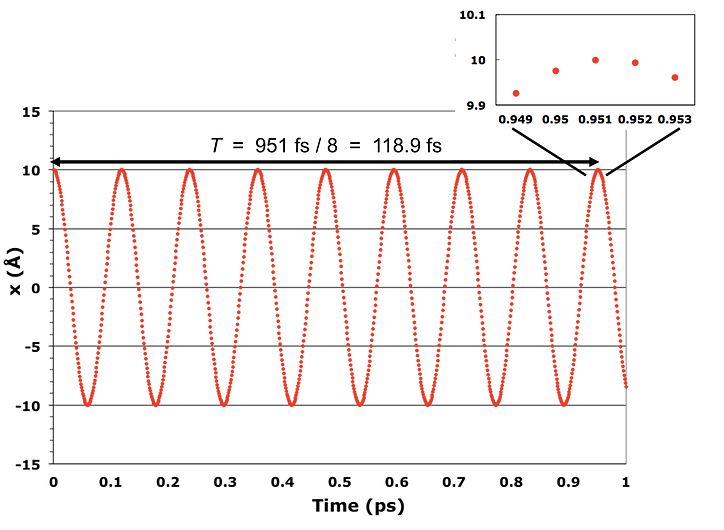
If the simulation accurately mimics the physical system, the oscillations in the bond length in the trajectory should have the same period as you calculated above. The figure at the right shows how the period can be determined by measuring the time interval between two peaks in the oscillation and dividing by the number of completed cycles.
For maximum accuracy, the two peaks should be as far apart in time as possible, so it is best to use the first and last peaks in the oscillation.
The following steps will allow you to measure the period:
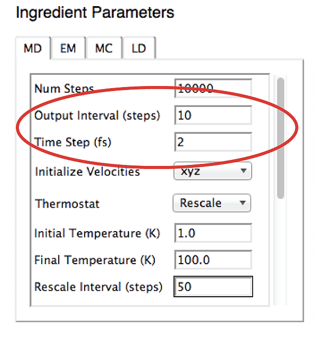
- The Sophia Bonds Plot and Energy Plot windows show values as a function of frame number. To convert frame number to time, you need to know the size of the time step and the output interval. This information can be found in the Sophia Recipe window. In the example at the right, each frame corresponds to 20 fs (2 fs per step x 10 steps per frame).
- The trajectory of Tutorial 1 begins with the bond stretched, so there is a peak in the bond length at t = 0. You can use the “zoom rectangle” control in the Sophia Energy Plot window to locate the time of the last peak in this plot. (See the zoom rectangle link if you don’t know how to zoom in on the peak.)
- What is the period of the bond length oscillations in this trajectory?
- Does the period of the simulation match the predicted period?
The predicted and observed periods should match. If they don’t, you have made a mistake. Carefully re-examine your calculations of both the theoretical period (Equation 2) and the period in the simulation.
2.4 Analyzing the simulation: energy conservation
A second criterion for an accurate MD simulation is that the total energy should be conserved. There are two aspects of this: the fluctuations in the total energy, and the long-time drift.
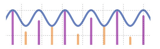
Use the “zoom rectangle” control in the Sophia Energy Plot window to expand the energy plot so you can inspect drift and fluctuations in the total energy (blue line) over the full length of the simulation. Your plot should look like the figure at the right, except it will cover the simulation from start to finish, and it will also show the values of the energy on the vertical axis.
- How large are the fluctuations in total energy? Express your answer as a fractional fluctuation \((E^{max}_{tot} - E^{min}_{tot}) / E^{max}_{tot}\) or a percent. To estimate the average energy, you can use the approximation \(E^{max}_{tot} \approx (E^{max}_{tot} + E^{min}_{tot}) / 2\)
- This is a very short simulation, so the total energy should not drift significantly upward or downward over the course of the simulation. Estimate the drift in total energy by comparing the tops of the peaks along the trajectory. Is it significant?