Tutorial 7 Simulated Annealing with Molecular Dynamics
7.1 Introduction
“Simulated annealing” refers to molecular mechanics algorithms aimed at optimizing the structure by first equilibrating it at a relatively high temperature T1, then cooling it gradually to a relatively low temperature T2. The basic idea is that high temperatures allow the system to explore conformational space relatively freely, and that it will move toward a minimum energy conformation as the temperature is lowered.
The name is derived from the metallurgical process of annealing, where a metal is heated to the point where its microcrystalline structure is broken, then cooled. The metal’s final properties (such as ductility) depend on the upper temperature, how long it is held at that temperature, the final temperature, and the cooling rate.
7.2 Set up universe
Create a new folder for your work on this tutorial.
Open Chimera, Launch Sophia, and initiate a new simulation with:
- PDB File: LJ10-2.pdb
- Force Field: Lennard-Jones
- FF Mod File: LJ_E0_0.1.frcmod
- Box length: 2 nm
- Non-bond cutoff: 1 nm
Click on Load Universe
In the UCSF Chimera window, click Actions / Atoms/Bonds / sphere to generate a space-filling model.
7.3 First annealing run
In the Sophia Recipe window:
Click on the MD tab (1) to be sure the active recipe is MD.
Click New (2). The default MD recipe will be loaded.
Click on the recipe (3). The blue band means that the recipe is active and can be edited.
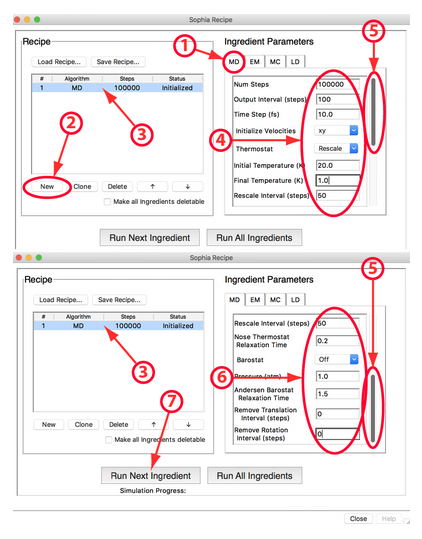
Edit the ingredient parameters (4). If necessary, drag the slider down (5) to expose the lower part of the window so you can edit the values there (6). Set the parameters as follows:
- Number of Steps: \(100000\)
- Output Interval: \(100\) steps
- Time Step: \(10\) fs
- Initialize Velocities: xy (keeps atoms in xy plane)
- Thermostat: Rescale
- Initial Temperature: \(20\) K
- Final Temperature: \(1\) K
- Rescale Interval: \(50\) steps
(Ignore the next four parameters)
- Remove Translation Interval: \(0\)
- Remove Rotation Interval: \(0\)
Be sure the recipe is still highlighted in blue (3).
Click on Run Next Ingredient (7).
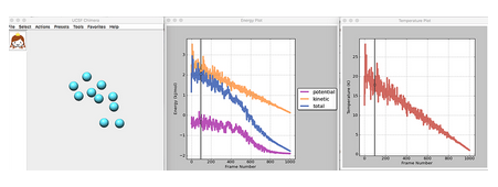
You should get results that look something like this (you can plot temperature by checking the appropriate box in the Viewer Controls window):
7.4 Analyze first annealing run
The trajectory you have just completed has the information you need to select appropriate values for T1 and T2, the upper and lower temperatures for simulated annealing on this system.
T1 needs to be high enough that the initial structure is completely broken up, so the system freely explores conformational space.
T2 needs to be low enough that the number and pattern of interatomic contacts does not change, so the system is at a minimum energy conformation. This will allow us to produce a collection of minimum energy conformations in a series of simulated annealing runs. If our annealing protocol is well designed, we should have a reasonable chance of finding the global minimum.
Scroll through the trajectory using the controls in the Trajectory Viewer window. Watch the atomic motions in the Chimera window. Note how the pattern of motions changes as the system is cooled, and how those changes are correlated with changes in the slope of the plot of the potential energy.
Write a short summary of the behavior of the system at different temperatures. You should include snapshots like the one above, to clarify the correlations between structure and temperature.
Use this description to select appropriate values of T1 and T2.
7.5 Set up and run annealing protocol
In the Sophia Recipe window, be sure that Recipe #1 is still highlighted in blue (3, in the figure above).
Click the Clone button to make a copy of the original recipe.
Click the box Make all ingredients deletable.
Be sure that recipe #1 is still highlighted in blue.
Click on the Delete button. Recipe #1 should disappear, and the new recipe will change from #2 to #1.
Click on the new recipe #1 so you can edit it.
Edit this recipe by changing the values of the initial and final temperatures to the values you selected for T1 and T2. Set the number of steps to 10,000 and the output interval to 10 steps, so you will again generate a trajectory with 1,000 frames.
While recipe #1 is highlighted in blue, click on the Clone button nine times, creating recipes #2 – #10.
Click on Run All Ingredients.
7.6 Analysis
The energy plot should look something like the frame below. You can expand the view as shown at the right by using the zoom rectangle option.
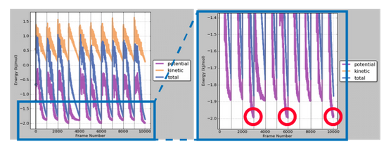
This particular simulation reached the global minimum energy structure three times (red circles), so the protocol had a success rate of 30%.
What was the success rate for your protocol?
7.7 Vary the length of the annealing protocol
In the Sophia Recipe window, delete recipes #2-10.
Clone recipe #1 (whose status is “Done”) to create recipe #2 (“Initialized”).
Delete recipe #1.
Following the procedure above, edit the recipe to change the number of steps from 10,000 to 100,000 and the output interval from 10 to 100, so you still get 1,000 frames per trajectory.
Make nine more clones of this recipe and run all ten of them.
What is the success rate now?
Create ten recipes with 1,000,000 steps each and an output interval of 1,000.
What is the success rate now?