Tutorial 4 MD Simulation on Two Atoms of Lennard-Jonesium

4.1 Introduction

“Lennard-Jonesium” is an idealized model for the interaction of two uncharged atoms. The interaction potential is described by the Lennard-Jones 6-12 potential. This potential combines the weakly attractive London dispersion forces and the strongly repulsive exchange (atomic overlap) forces.

This tutorial carries out an MD simulation on two atoms of Lennard-Jonesium, restricted to move in only one dimension. This will introduce you to the dynamic behavior of non-covalently-linked atoms, and to the Lennard-Jones potential.

For two atoms separated by a distance r,

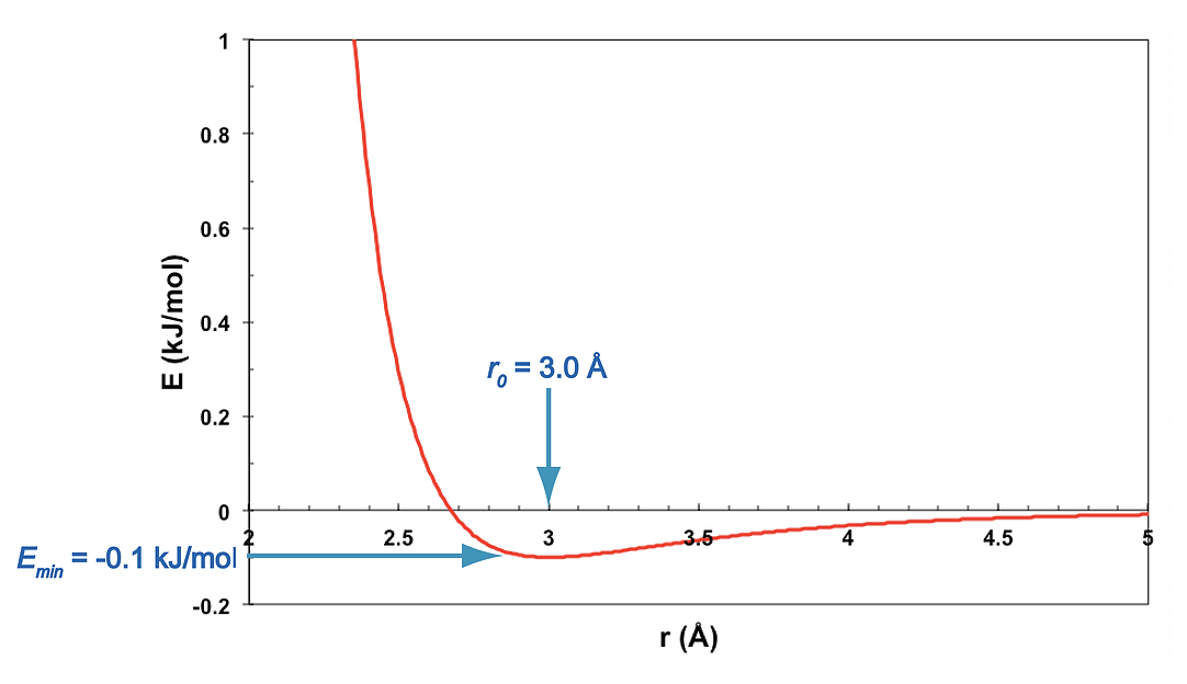
\[\begin{equation} E_{LJ}(r) = E_0 \left[\left(\frac{r_0}{r}\right)^{12} - 2\left(\frac{r_0}{r}\right)^6\right] \tag{4.1} \end{equation}\]

In this exercise, the ideal distance is \(r_0 = 3Å\), and the well depth is \(E_0 = 0.1\) kJ/mol.

As seen in the graph, the negative r-6 potential is weakly attractive, and it dominates when \(r > r_0\), the ideal contact distance. The positive r-12 term is strongly repulsive and dominates when \(r < r_0\).

4.2 Getting ready

Create a new folder for your work on this tutorial. Download the following files and put them in that folder:

• PDB File: LJ2.pdb
• FF Mod File: LJ_E0_0.1.frcmod
• Recipe: LJ2_recipe.json

4.3 Prediction

An MD simulation mimics the behavior of real masses, in this case two atoms acting under the influence of the Lennard-Jones force between them. At the start of the simulation (\(t = 0\)), the two atoms are at rest on the x-axis, separated by a distance of \(8Å\). Their motion is confined to that single dimension: throughout the simulation, \(y = 0\) and \(z = 0\). What do you think they will do as time passes?

To predict the behavior, just ask yourself, “What would two real masses do if they were sitting, at rest, on the Lennard-Jones energy surface shown above, and then released?” You are to express your prediction by describing the trajectory of the system, drawing a graph showing \(r(t)\).

What’s important here is for you to think about the system for a while and make a guess about its behavior. It’s not important that your prediction be right. You will learn more from this simulation if you make a prediction – even if it’s wrong – than you will if you simply run it without thinking about what might happen.

The simplest way to think about this system is to imagine one atom as a ball sitting on the van der Waals energy surface produced by the other atom, as in the figure. The position of the single ball (r) represents the distance between the two atoms. (This is an example of a simple coordinate transformation. In this case the motions of the two atoms, \(x_1(t)\) and \(x_2(t)\) are reduced to a single coordinate, \(r(t)\). You may find it easier to think about the motion of this “ball” in a fixed potential than it is to think about the motions of the two atoms.)

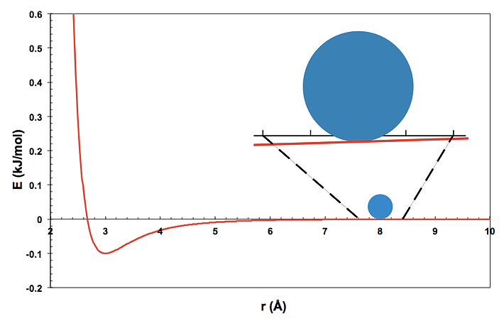
Gravity pulls the ball downward. If you answer the following questions, you should be able to predict how the ball will move, that is, how the distance between the two atoms will change as time passes.

• At the start of the simulation, do you expect the atoms to move, or not? In which direction? (That is, do you expect the two atoms to move toward one another, or away from one another, or to stay fixed?)

• Do you expect the motion to be monotonic (in one direction, forever)? Or do you expect the motion to reverse direction? If so, how far will the atoms go before changing direction?

• And what will happen then? Will the atoms return to their original positions or not?

• Will the motion be periodic, or not? If it is, do you expect it to be damped by friction? Will the atoms eventually come to rest? If so, where?

Once you’ve made your final guess, make your prediction semi-quantitative by sketching a rough graph of \(r(t)\), that is, with time on the horizontal axis and r on the vertical axis. Again, it doesn’t matter whether your guess is right or not – what’s important is for you to think about the likely behavior of the system. This will help you understand the results of the simulation, once it’s been run.

4.4 Running the simulation

Throughout this tutorial, avoid rotating the structure in the Chimera window. This is a one-dimensional system with \(y = 0\) and \(z = 0\) for all atoms in the trajectory. If you rotate the structure, you will not be able to see motion in the x direction correctly. You can reset the view by clicking on the Reset View button in the Chimera sidebar.

1. Run an MD simulation in Sophia using the input files listed above. (If you need help setting up and running the simulation, follow the instructions in Tutorial 1). The recipe should produce a simulation with

   • a box length of \(10\) nm
   • a cutoff of \(1\) nm
   • a stepsize of \(1\) fs
   • \(10000000\) steps (\(10\) ns)
   • an output interval of \(100\) steps (\(100\) fs)

2. Create a plot of \(r(t)\), the distance between the two atoms using Chimera’s distance measurement tool and the Sophia Trajectory Viewer window (refer to Tutorial 1 for detailed instructions).

4.5 Analysis

3. Compare the plot of \(r(t)\) with the sketch you made of your predicted behavior of \(r(t)\). Write a brief description of any differences, explaining the reasoning behind your prediction, and the reason the system behaved differently than you expected.

4. Examine the time-dependence of \(E_{pot}\), \(E_{kin}\) and \(E_{tot}\). Explain the behavior.

5. Look at \(E_{tot}\) in detail. How well is it conserved?

6. What is the period of the motion?

4.6 Challenge

Can you come up with an analytic expression for the period as a function of the Lennard-Jones parameters \(E_0\) and \(r_0\), and the initial position \(r(t=0)\)? This is a difficult problem, but it has a solution.

Show that the period predicted by your analytic expression is equal to the period observed in the simulation.